1、实验目的
(1) 学习“NOTEARS/ PC/GraN-DAG”等因果发现算法在python中的使用与实现;
(2) 学习AMOS软件,计算因果效应
(3) 学会用Grid Search/BOHB等方法或工具进行超参数调优
(4) 通过多项指标比较比较算法效果
(5) 结果可视化与展示。
2、实验准备
1、准备好python环境和编译器软件(PyCharm或Visual Studio Code);
2、自行在网络资源中找到“NOTEARS/ PC/GraN-DAG”对应的python代码(推荐渠道:
1.NOTEARS官方项目https://github.com/xunzheng/notears;
2.GraN-DAG官方项目https://github.com/lihebi/GraN-DAG-nodata;
3.华为诺亚实验室集成工具库
https://github.com/huawei-noah/trustworthyAI/tree/master/gcastle),并完成算法所需要python库的安装;
注:上课演示以NOTEARS为例,先保证该算法配置完成
3、根据教程安装好AMOS软件https://blog.csdn.net/2303_81888702/article/details/135410867;
4、提前熟悉实验材料(及其中涉及的概念)和所对应的算法代码,可借助大模型平台(如:ChatGPT/通义千问等)。
NOTEARS的官方资源和AMOS安装文件已分别打包为“notears-master.zip”、“Amos28.zip”。
3、实验原理
一、因果发现:
因果发现,即从纯观测数据中发现并获取因果关系。
因果模型本质是反应变量之间的因果关系,比如我们有两个变量“吃饭”与“饱足”,我们知道二者是相关的,那么我们如何描述两个变量间的因果关系呢?其实通过一种有向的描述即可,我们会发现:吃饭会导致饱足,但是饱足不会导致吃饭。因此吃饭是饱足的因。我们可以表述为“吃饭-->饱足”,所以我们可以发现,这本质上是一个有向无环的图模型(DAG)。所以如果我们可以通过一组变量写出其对应的DAG(专业术语是马尔可夫相容),那么我们就可以表达变量间的因果关系。
 |
|---|
因果发现是一种统计学和机器学习的分支,旨在识别哪些变量是其他变量的原因,哪些是结果。由于直接观察因果关系通常是困难的,尤其是在自然和社会科学中,因果发现方法利用统计依赖性、干预数据(如果有的话)、背景知识以及特定的算法和技术来估计这些关系。
当前主要有四种因果结构发现的方法:基于约束的方法、基于分数的方法、利用结构不对称性的方法和利用各种形式的干预的方法。每种方法可进一步被分为通过基于组合/搜索的算法和通过基于连续优化的算法。这些方法也可以被分为局部(local)即每次测试一条边,和全局(global)即测试整张图。
**二、**PC
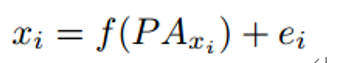
PC (Hoyer等人(2008))使用加性噪声模型进行因果发现,并提供了线性非高斯因果发现框架的推广,以处理变量具有加性噪声的非线性函数依赖。它提到非线性因果关系通常有助于打破观察变量之间的对称性,并有助于确定因果方向。PC假设观测变量的数据生成过程如下面的公式所示,其中变量xi是其父变量的函数,而噪声项ei是独立的加性噪声。
**三、**NOTEARS
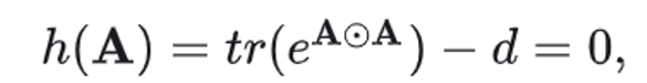
NOTEARS (Zheng et al .(2018))是第一个将组合图搜索问题重建为连续优化问题的,并且许多方法改造了该方法的主要贡献即无环性惩罚。强制无环性的函数/惩罚 h 为:
将传统的组合优化问题(左)转化为连续程序(右)
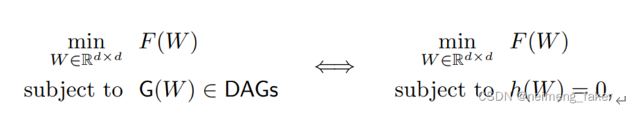
使用增广拉格朗日的标准机制,转换为无约束问题

**四、**GraN-DAG
基于梯度的神经DAG学习(GraN-DAG)是一种基于分数的结构学习方法,它使用神经网络(nn)来处理非线性因果关系(Lachapelle et al .(2019))。它使用随机梯度方法来训练神经网络,以提高可扩展性并允许隐式正则化。它基于NOTEARS为神经网络制定了一种新的非周期性表征(Zheng et al .(2018))。为了确保非线性模型中的非周期性,它使用了一个类似于NOTEARS的参数,并首先在神经网络路径级别应用它,然后在图路径级别应用它。对于正则化,GraN-DAG使用一个称为初步邻居选择(PNS)的过程来为每个变量选择一组潜在的父变量。它使用最后的修剪步骤来去除假边。该算法主要适用于非线性高斯加性噪声模型。
五、结构因果模型:
结构因果模型由 Pearl 提出,其将所有考虑的变量组织成一个有向无环图,也称作因果图 (causal graph),记作 G = (V,E) ,每个节点代表一个变量,一条由X 指向Y 的边代表X对Y有直接的因果作用。
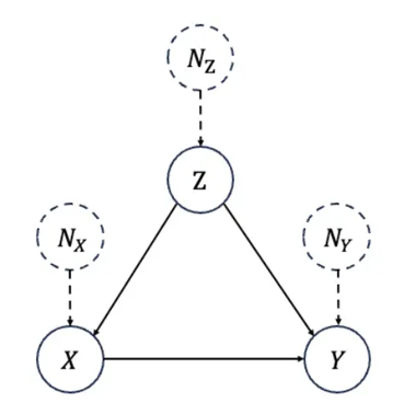
节点的值由外生变量 (exogenous variable) 和所有直接父节点变量通过结构方程 (structural equations) 唯一确定。
六、超参数调优
https://zhuanlan.zhihu.com/p/590823641
模型参数:这些是由模型从给定的数据中估计出来的参数。例如,一个深度神经网络的权重。
模型超参数:这些是不能由模型从给定数据中估计的参数,超参数被用来估计模型的参数,例如,深度神经网络的学习率。
超参数调优的主要方法:
手动超参数调优:包括通过手动方式来实验不同的超参数集。
随机搜索(Random Search):在随机搜索方法中,我们为超参数创建了拥有很多可能值的网格。每次迭代都从这个网格中尝试随机的超参数组合,记录性能,最后得到最佳性能的超参数组合。
**网格搜索(Grid Search):**在网格搜索法中,我们为超参数创建了一个可能值的网格。每次迭代都以特定的顺序尝试超参数的组合。它在每一个可能的超参数组合上拟合模型并记录模型的性能。最后,它返回具有最佳超参数的最佳模型。
贝叶斯优化:为模型调整和寻找合适的超参数是一种优化问题。我们希望通过改变模型参数来最小化我们模型的损失函数。贝叶斯优化帮助我们通过最少的步骤中找到最小的点。贝叶斯优化还使用了采集函数(Acquisition Funtion),将采样引向有可能比当前最佳观察结果更好的区域。
4、实验内容
1、在python上实现NOTEARS,并通过生成数据对算法进行调参,之后将调优后的算法应用到给定数据,最后得到学习到的DAG。
exp_linear/graph00000_data00000_X _.csv
其中给定数据的已知信息如下:
真实DAG的边缘数量为14-18
graph_type = 'ER';sem_type = 'gauss';w_ranges = ((-2.0, -0.5), (0.5, 2.0)); noise_scale = np.ones(d)
2、将学习到的DAG应用到AMOS中进行计算因果效应,观察拟合指标是否达标,若不达标说明算法从数据中学习到的DAG与实际不符,需要重新进行步骤1。要求最终的AMOS指标处于合理范围。
3、基于分组给定三组不同分布的数据(包含三个文件),此时已知真实DAG。要求分别在三组数据上应用三个算法,并通过评价指标比较算法性能。
数据文件的具体分配参照“数据集分配.xlsx”
要用的数据文件格式如下:
exp_nonlinear1/ graph0000x_W_true .csv
exp_nonlinear1/graph0000x_data0000y_X .csv
exp_nonlinear2/ graph0000x_W_true .csv
exp_nonlinear2/graph0000x_data0000y_X .csv
exp_nonlinear3/ graph0000x_W_true .csv
exp_nonlinear3/graph0000x_data0000y_X .csv
其中x,y的值为0或1
5、实验要求
1.通过python实现PC/NOTEARS/GraN-DAG算法的运行。
2.通过使用超参数调优策略(网格搜索或贝叶斯策略或其它工具,如BOHB)参数调整理解优化算法中各个参数的意义。
3.通过NOTEARS学习未知真实DAG数据集中的DAG,并应用AMOS软件计算因果效应.
4.提交NOTEARS最后的超参数、因果图以及各路径的因果效应。
6、实验过程
展示主要的实验过程(整体流程+具体进行设计的地方+实验测试过程)
文字+图片(如:代码截图)
A 未知真实DAG数据集:
主要体现两部分内容:
(1)超参数调优代码设计
数据生成:
from notears import linear, utils
import numpy as np
from tqdm import tqdm
from collections import defaultdict
import os


def main():
    utils.set_random_seed(123)
    # 生成图的数量
    num_graph = 2
    # 每个图对应生成数据集的份数
    num_data_per_graph = 2
    # 生成数据的保存地址
    save_data_path = r"data"
    # n-生成的数据量,多少条数据;d-生成图/生成数据的维度,几个变量;s0-生成图的边数;
    # graph_type-生成图的类型(ER, SF, BP);sem_type-生成数据的分布类型(线性:gauss, exp, gumbel, uniform, logistic, poisson/非线性:mlp, mim, gp, gp-add)
    n, d, s0, graph_type, sem_type = 200, 7, 14, 'ER', 'gauss'
    n1, d1, s1, graph_type1, sem_type1 = 30, 3, 2, 'SF', 'mlp'

    # 线性数据例子
    # w_ranges-参数的数据范围
    w_ranges = ((-2.0, -0.5), (0.5, 2.0))
    # noise_scale-加性噪声的范围
    noise_scale = np.ones(d)
    # 生成数据存放文件夹的名称
    expt_name = 'equal_var'
    run_expt(save_data_path, num_graph, num_data_per_graph, n, d, s0, graph_type, sem_type, w_ranges, noise_scale, expt_name)

    # 非线性数据例子
    w_ranges = ((-2.0, -1.1), (1.1, 2.0))
    noise_scale1 = [1., 0.15, 0.2]
    expt_name = 'large_a'
    #run_expt_(save_data_path, num_graph, num_data_per_graph, n1, d1, s1, graph_type1, sem_type1, w_ranges, noise_scale1, expt_name)

# 线性
def run_expt(save_data_path, num_graph, num_data_per_graph, n, d, s0, graph_type, sem_type, w_ranges, noise_scale, expt_name):
    # os.mkdir(expt_name)
    # os.chmod(expt_name, 0o777)
    # perf = defaultdict(list)
    noise_scale  =np.array(noise_scale)
    for ii in tqdm(range(num_graph)):
        # B_true-生成因果图的0-1邻接矩阵
        B_true = utils.simulate_dag(d, s0, graph_type)
        W_true = utils.simulate_parameter(B_true, w_ranges=w_ranges)
        B_true_fn = os.path.join(save_data_path, expt_name, f'graph{ii:05}_W_true.csv')
        np.savetxt(B_true_fn, B_true, delimiter=',')
        for jj in range(num_data_per_graph):
            # X = utils.simulate_linear_sem(W_true, n, sem_type, noise_scale=noise_scale)
            X = utils.simulate_linear_sem(W_true, n, sem_type, noise_scale=noise_scale)
            X_fn = os.path.join(save_data_path, expt_name, f'graph{ii:05}_data{jj:05}_X.csv')
            np.savetxt(X_fn, X, delimiter=',')

# 非线性
def run_expt_(save_data_path, num_graph, num_data_per_graph, n, d, s0, graph_type, sem_type, noise_scale, expt_name):
    noise_scale = np.array(noise_scale)
    for ii in tqdm(range(num_graph)):
        B_true = utils.simulate_dag(d, s0, graph_type)
        B_true_fn = os.path.join(save_data_path, expt_name, f'graph{ii:05}_W_true.csv')
        np.savetxt(B_true_fn, B_true, delimiter=',')
        for jj in range(num_data_per_graph):
            X = utils.simulate_nonlinear_sem(B_true, n, sem_type, noise_scale=noise_scale)
            X_fn = os.path.join(save_data_path, expt_name, f'graph{ii:05}_data{jj:05}_X.csv')
            np.savetxt(X_fn, X, delimiter=',')


if __name__ == '__main__':
    main()
网格搜索代码:
from notears import linear, nonlinear, utils
import numpy as np
with open(r'D:\Desktop\TBFILE\学习\群体智能\群体智能第二次实验\notears-master\data\equal_var\graph00001_W_true.csv') as f:
line = f.readline()
data_array = []
while line:
num = list(map(float, line.split(',')))
data_array.append(num)
line = f.readline()
B_true = np.array(data_array)
with open(r'D:\Desktop\TBFILE\学习\群体智能\群体智能第二次实验\notears-master\data\equal_var\graph00001_data00001_X.csv') as f:
line = f.readline()
data_array = []
while line:
num = list(map(float, line.split(',')))
data_array.append(num)
line = f.readline()
X = np.array(data_array)
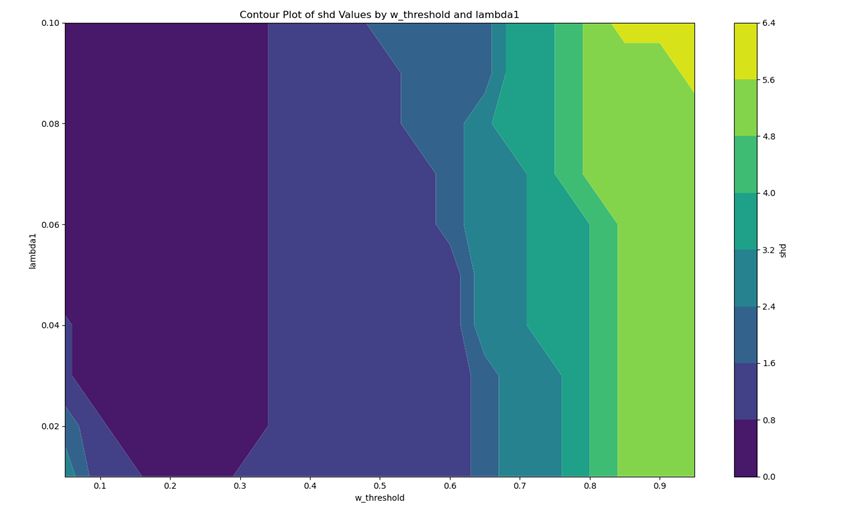
param_dist = {
# "max_iter":[100, 200, 300, 400, 500],
"w_threshold":[0.05, 0.1, 0.15, 0.2, 0.25, 0.3, 0.35, 0.4, 0.45, 0.5, 0.55, 0.6, 0.65, 0.7, 0.75, 0.8, 0.85, 0.9, 0.95],
# "lambda0":[0.001, 0.003, 0.004, 0.005, 0.007, 0.009, 0.011, 0.013, 0.015, 0.017, 0.019, 0.021, 0.023, 0.025],
"lambda1":[0.01, 0.02, 0.03, 0.04, 0.05, 0.06, 0.07, 0.08, 0.09, 0.1],
}
# MI = param_dist.get("max_iter")
WT = param_dist.get("w_threshold")
L1 = param_dist.get("lambda1")
result = []
for i in range(len(L1)):
for j in range(len(WT)):
#notears
lambda1 = L1[i]
w_threshold = WT[j]
W_notears = linear.notears_linear(X, lambda1=lambda1, loss_type='l2',max_iter=300,
w_threshold=w_threshold)
assert utils.is_dag(W_notears)
#eval
B_notears = (W_notears !=0)
acc = utils.count_accuracy(B_true, B_notears)
print("----------------------------------")
print("lambda1:",L1[i],"w_threshold:",WT[j])
ret = [L1[i],WT[j]]
v_met = list(acc.values())
print("fdr|tpr|shd|nnz")
print(v_met)
ret += v_met
result.append(ret)
import csv
# 创建csv writer对象
with open(r'data\equal_var\res_save\r_l11.csv', 'w', newline='') as file1:
writer1 = csv.writer(file1)
# 写入数据
for row in result:
writer1.writerow(row)
# 数据
data = [["lambda1:","w_threshold:"] + list(acc.keys())]+result
# 创建csv writer对象
with open(r'data\equal_var\res_save\d_l11.csv', 'w', newline='') as file2:
writer2 = csv.writer(file2)
# 写入数据
for row in data:
writer2.writerow(row)(2)测试过程
体现测试的过程,至少将两次测试不成功(即:应用AMOS计算因果效应时,拟合指标不达标,学习到的因果图不准确)的例子进行呈现——此时预设的边的数量,超参数,结果图(因果图+AMOS计算结果)
试验过程:
| Lambda1:0.01 w_threshold:0.2 **边的数量:**16 |
|---|
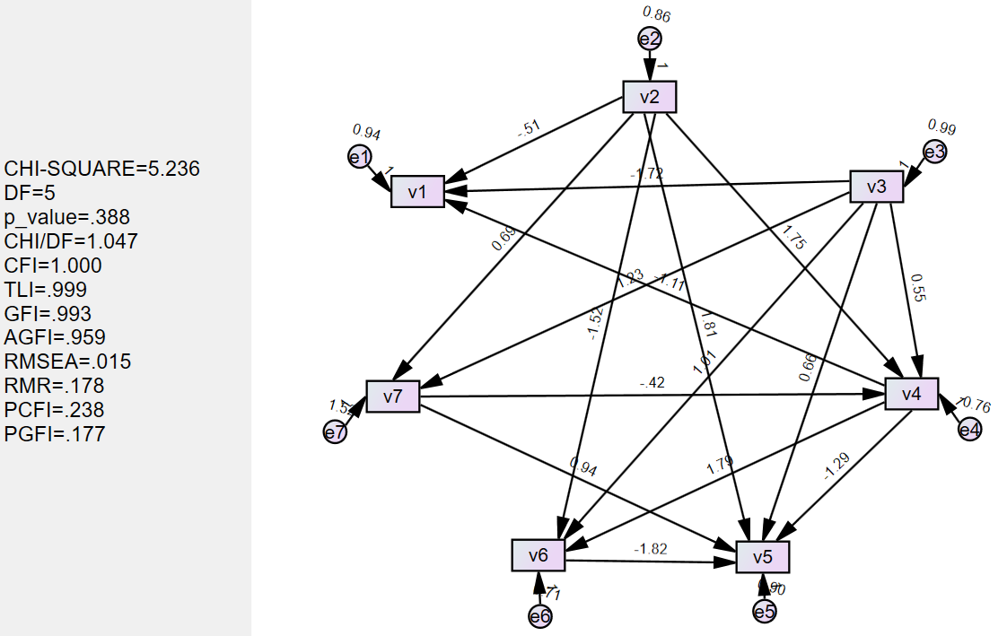 |
| Lambda1:0.01 w_threshold:0.2 **边的数量:****15 |
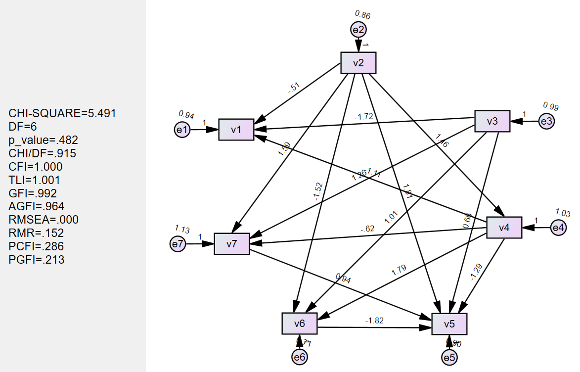 |
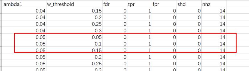
最优解:
| **最优:**Lambda1:0.05 w_threshold:0.1 边的数量:16 |
|---|
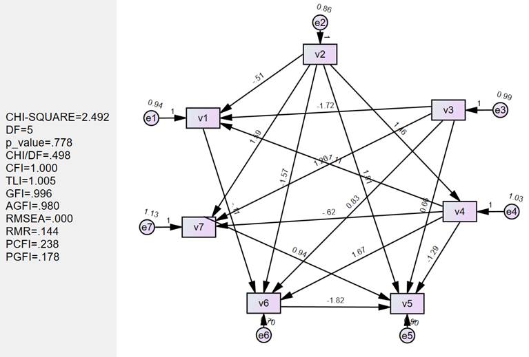 |
B 已知真实DAG数据集:
主要体现不同算法在不同数据集上的超参数调优过程及对比过程
要求对最后的比较结果作分析和评述
NOTEARS
网格搜索超参数优化:
import torch
import torch.nn as nn
import numpy as np
import csv
from notears.locally_connected import LocallyConnected
from notears.lbfgsb_scipy import LBFGSBScipy
from notears.trace_expm import trace_expm
import notears.utils as ut
from notears import linear, nonlinear, utils


# Define NotearsMLP and NotearsSobolev classes here (as provided)

def squared_loss(output, target):
    n = target.shape[0]
    loss = 0.5 / n * torch.sum((output - target) ** 2)
    return loss


def dual_ascent_step(model, X, lambda1, lambda2, rho, alpha, h, rho_max):
    h_new = None
    optimizer = LBFGSBScipy(model.parameters())
    X_torch = torch.from_numpy(X)
    while rho < rho_max:
        def closure():
            optimizer.zero_grad()
            X_hat = model(X_torch)
            loss = squared_loss(X_hat, X_torch)
            h_val = model.h_func()
            penalty = 0.5 * rho * h_val * h_val + alpha * h_val
            l2_reg = 0.5 * lambda2 * model.l2_reg()
            l1_reg = lambda1 * model.fc1_l1_reg()
            primal_obj = loss + penalty + l2_reg + l1_reg
            primal_obj.backward()
            return primal_obj

        optimizer.step(closure)
        with torch.no_grad():
            h_new = model.h_func().item()
        if h_new > 0.25 * h:
            rho *= 10
        else:
            break
    alpha += rho * h_new
    return rho, alpha, h_new


def notears_nonlinear(model: nn.Module,
                      X: np.ndarray,
                      lambda1: float = 0.,
                      lambda2: float = 0.,
                      max_iter: int = 100,
                      h_tol: float = 1e-8,
                      rho_max: float = 1e+16,
                      w_threshold: float = 0.3):
    rho, alpha, h = 1.0, 0.0, np.inf
    for _ in range(max_iter):
        rho, alpha, h = dual_ascent_step(model, X, lambda1, lambda2,
                                         rho, alpha, h, rho_max)
        if h <= h_tol or rho >= rho_max:
            break
    W_est = model.fc1_to_adj()
    W_est[np.abs(W_est) < w_threshold] = 0
    return W_est


def main():
    torch.set_default_dtype(torch.double)
    np.set_printoptions(precision=3)
    ut.set_random_seed(123)

    # Load observational data from CSV file
    X = np.genfromtxt(
        r'D:\Desktop\TBFILE\学习\群体智能\群体智能第二次实验\exp_nonlinear_3\graph00001_data00000_X.csv',
        delimiter=',', skip_header=1)
    # Load ground truth DAG from CSV file
    B_true = np.genfromtxt(
        r'D:\Desktop\TBFILE\学习\群体智能\群体智能第二次实验\exp_nonlinear_3\graph00001_W_true.csv',
        delimiter=',')

    d = X.shape[1]

    # Hyperparameters for grid search
    param_dist = {
        "w_threshold": [0.05,0.10,0.15,0.2, 0.25, 0.3, 0.35, 0.4, 0.45, 0.5],
        "lambda1": [0.01, 0.02, 0.03,  0.04, 0.05],
        "lambda2": [0.01, 0.02, 0.03, 0.04, 0.05]
    }

    WT = param_dist["w_threshold"]
    L1 = param_dist["lambda1"]
    L2 = param_dist["lambda2"]

    result = []
    for lambda1 in L1:
        for lambda2 in L2:
            for w_threshold in WT:
                model = nonlinear.NotearsMLP(dims=[d, 10, 1], bias=True)
                W_est = notears_nonlinear(model, X, lambda1=lambda1, lambda2=lambda2, w_threshold=w_threshold)

                # Ensure W_est is a DAG
                if not ut.is_dag(W_est):
                    continue  # Skip this combination if it's not a DAG

                # Save results for each combination
                ret = [lambda1, lambda2, w_threshold]
                ret += list(ut.count_accuracy(B_true, W_est != 0).values())
                result.append(ret)

                # Print results for debugging
                print(f"lambda1: {lambda1}, lambda2: {lambda2}, w_threshold: {w_threshold}")
                print("fdr|tpr|shd|nnz")
                print(list(ut.count_accuracy(B_true, W_est != 0).values()))

    # Save results to CSV files
    headers = ["lambda1", "lambda2", "w_threshold"] + list(ut.count_accuracy(B_true, W_est != 0).keys())
    data = [headers] + result

    with open(
            r'D:\Desktop\TBFILE\学习\群体智能\群体智能第二次实验\exp_nonlinear_3\grid_search_results1.csv',
            'w', newline='') as file:
        writer = csv.writer(file)
        for row in data:
            writer.writerow(row)


if __name__ == '__main__':
    main()
    print('done')
优化结果:
| lambda1 | lambda2 | w_threshold | fdr | tpr | fpr | shd | nnz | |
|---|---|---|---|---|---|---|---|---|
| exp_nonlinear_1 | 0.02 | 0.01 | 0.35 | 0.04 | 0.888889 | 0.019608 | 4 | 25 |
| exp_nonlinear_2 | 0.01 | 0.02 | 0.4 | 0.058824 | 0.592593 | 0.019608 | 11 | 17 |
| exp_nonlinear_3 | 0.01 | 0.02 | 0.25 | 0.2 | 0.888889 | 0.117647 | 9 | 30 |
GraN-DAG
网格搜索超参数优化:
from castle.common import GraphDAG
from castle.metrics import MetricsDAG
from castle.algorithms import GraNDAG
import numpy as np
import pandas as pd
import itertools

# Set random seed for reproducibility
np.random.seed(42)

# Load observational data from CSV file
X = np.genfromtxt(
    r'D:\Desktop\TBFILE\学习\群体智能\群体智能第二次实验\exp_nonlinear_1\graph00001_data00000_X.csv',
    delimiter=',', skip_header=1)

# Load ground truth DAG from CSV file
B_true = np.genfromtxt(
    r'D:\Desktop\TBFILE\学习\群体智能\群体智能第二次实验\exp_nonlinear_1\graph00001_W_true.csv',
    delimiter=',')

# Normalize data
normalize = True
if normalize:
    X_mean = np.mean(X, axis=0, keepdims=True)
    X_std = np.std(X, axis=0, keepdims=True)
    X = (X - X_mean) / X_std

# Check for NaN values in the data
if np.isnan(X).any():
    raise ValueError("Input data contains NaN values. Please check the data preprocessing steps.")

# Define hyperparameter grid
param_grid = {
    'model_name': ['NonLinGauss'],
    'nonlinear': ['leaky-relu'],
    'optimizer': ['sgd'],
    'norm_prod': ['paths'],
    'device_type': ['cpu'],
    'random_seed': [42],
    'normalize': [normalize],
    'input_dim': [X.shape[1]],
    'hidden_num': [2, 3,4],
    'hidden_dim': [10, 20, 30],
    'batch_size': [64,128],
    'lr': [0.0001],
    'iterations': [1000]
}

# Create a list to store results
results = []

# Perform grid search
keys, values = zip(*param_grid.items())
for v in itertools.product(*values):
    params = dict(zip(keys, v))

    try:
        # Create and train GraNDAG instance
        gnd = GraNDAG(**params)
        gnd.learn(data=X)

        # Evaluate the learned DAG
        mm = MetricsDAG(gnd.causal_matrix, B_true)

        # Store results
        result = params.copy()
        result.update(mm.metrics)
        results.append(result)

        # Print current result
        print(f"Evaluated params: {params}")
        print(f"Metrics: {mm.metrics}\n")

    except ValueError as e:
        print(f"Error with params: {params}")
        print(e)
        continue

# Save results to CSV
results_df = pd.DataFrame(results)
results_df.to_csv(r'D:\Desktop\TBFILE\学习\群体智能\群体智能第二次实验\exp_nonlinear_1\pc_results.csv',
                  index=False)

print("Grid search completed. Results saved to CSV.")
优化结果
| hidden_num | hidden_dim | batch_size | fdr | tpr | fpr | shd | nnz | |
|---|---|---|---|---|---|---|---|---|
| exp_nonlinear_1 | 2 | 10 | 128 | 0.5556 | 0.1481 | 0.098 | 28 | 9 |
| exp_nonlinear_2 | 4 | 10 | 64 | 0.6667 | 0.1481 | 0.1569 | 28 | 12 |
| exp_nonlinear_3 | 3 | 20 | 64 | 0.8 | 0.0741 | 0.1569 | 30 | 10 |
PC
贝叶斯搜索超参数优化:
import pandas as pd
import numpy as np
from castle.algorithms import PC
from castle.metrics import MetricsDAG
from bayes_opt import BayesianOptimization
import logging

# Set up logging
logging.basicConfig(level=logging.INFO)
logger = logging.getLogger(__name__)

# 读取CSV数据文件
data_path = r'D:\Desktop\TBFILE\学习\群体智能\群体智能第二次实验\exp_nonlinear_3\graph00001_data00000_X.csv'
data = pd.read_csv(data_path)

# 读取真实的因果图
true_graph_path = r'D:\Desktop\TBFILE\学习\群体智能\群体智能第二次实验\exp_nonlinear_3\graph00001_W_true.csv'
true_dag = pd.read_csv(true_graph_path, header=None).values

# 将数据转换为numpy数组
X = data.values

# 定义目标函数
def objective(alpha):
    try:
        # 设置新的alpha值并初始化PC算法
        pc = PC(variant='stable', alpha=alpha)

        # 学习因果结构
        pc.learn(X)

        # 评估学习到的因果矩阵
        met = MetricsDAG(pc.causal_matrix, true_dag)

        # 记录SHD值
        shd = met.metrics['shd']

        logger.info(f'Alpha: {alpha}, SHD: {shd}')

        # 返回SHD的负值,因为贝叶斯优化是一个最大化器,我们希望最小化SHD
        return -shd
    except Exception as e:
        logger.error(f"Error with alpha: {alpha}")
        logger.error(e)
        return -float('inf')

# 设置贝叶斯优化的参数范围
pbounds = {'alpha': (0.01, 0.1)}

# 初始化贝叶斯优化器
optimizer = BayesianOptimization(
    f=objective,
    pbounds=pbounds,
    random_state=42
)

# 执行优化过程
optimizer.maximize(n_iter=20)

# 获取最佳参数
best_alpha = optimizer.max['params']['alpha']
best_shd = -optimizer.max['target']

print(f'\nBest alpha: {best_alpha}, with SHD: {best_shd}')
优化结果:
| pc | alpha | fdr | tpr | fpr | shd | nnz |
|---|---|---|---|---|---|---|
| exp_nonlinear_1 | 0.04370861069626263 | 0.2857 | 0.3704 | 0.0784 | 19 | 14 |
| exp_nonlinear_2 | 0.09556428757689246 | 0.4118 | 0.3704 | 0.1373 | 20 | 17 |
| exp_nonlinear_3 | 0.04370861069626263 | 0.3889 | 0.4074 | 0.1373 | 18 | 18 |
8、结果展示
A.未知真实DAG数据集:
(0)超参数优化图/或表格
体现超参数优化过程
 |
|---|
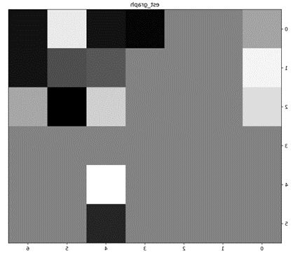
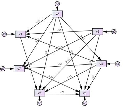
(1)因果图:
坐标点图、连线图或其他形式,可自行设计
 |
 |
|---|---|
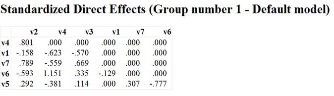
(2)AMOS计算结果图:
截图呈现
| **最优:**lambda1:0.05 w_threshold:0.1 |
|---|
|
| 路径效应计算结果截图,包含总效应/直接效应/间接效应 |
|---|
 |
 |
 |
B.已知真实DAG数据集:
(1)因果图:
给出各个算法在不同数据集上学习到的最优DAG
 |
|---|
(2)算法性能比较结果呈现:
通过表格呈现比较结果
exp_nonlinear_1:
| fdr | tpr | fpr | shd | nnz | |
|---|---|---|---|---|---|
| NOTEARS | 0.04 | 0.888889 | 0.019608 | 4 | 2 |
| GraN-DAG | 0.5556 | 0.1481 | 0.098 | 28 | 9 |
| PC | 0.4118 | 0.3704 | 0.1373 | 20 | 17 |
exp_nonlinear_2:
| fdr | tpr | fpr | shd | nnz | |
|---|---|---|---|---|---|
| NOTEARS | 0.058824 | 0.592593 | 0.019608 | 11 | 17 |
| GraN-DAG | 0.6667 | 0.1481 | 0.1569 | 28 | 1 |
| PC | 0.4118 | 0.3704 | 0.1373 | 20 | 17 |
exp_nonlinear_3:
| fdr | tpr | fpr | shd | nnz | |
|---|---|---|---|---|---|
| NOTEARS | 0.2 | 0.888889 | 0.117647 | 9 | 30 |
| GraN-DAG | 0.8 | 0.0741 | 0.1569 | 30 | 10 |
| PC | 0.3889 | 0.4074 | 0.1373 | 18 | 18 |
通过上面表格比较可知:
NOTEARS 算法在所有三个数据集上都表现最佳,SHD 最低,能够更准确地学习到真实的因果关系结构
而GraN-DAG、PC算法表现不佳的原因可能是因为该数据集不适合这两种算法,从而导致这两种算法不能很好的学习因果关系结构